Prettier LowLevelCallables with Numba JIT and decorators

In my recent post, I extolled the virtues of SciPy 0.19’s LowLevelCallable. I did lament, however, that for generic_filter, the LowLevelCallable interface is a good deal uglier than the standard function interface. In the latter, you merely need to provide a function that takes the values within a pixel neighbourhood, and outputs a single value — an arbitrary function of the input values. That is a Wholesome and Good filter function, the way God intended.

In contrast, a LowLevelCallable takes the following signature:

int callback(double *buffer, intptr_t filter_size, 
             double *return_value, void *user_data)

That’s not very Pythonic at all. In fact, it’s positively Conic (TM). For those that don’t know, pointers are evil, so let’s aim to avoid their use.

“But Juan!”, you are no doubt exclaiming. “Juan! Didn’t you just tell us how to use pointers in Numba cfuncs, and tell us how great it was because it was so fast?”

Indeed I did. But it left a bad taste in my mouth. Although I felt that the tradeoff was worth it for such a phenomenal speed boost (300x!), I was unsatisfied. So I started immediately to look for a tidier solution. One that would let me write proper filter functions while still taking advantage of LowLevelCallables.

It turns out Numba cfuncs can call Numba jitted functions, so, with a little bit of decorator magic, it’s now ludicrously easy to write performant callables for SciPy using just pure Python. (If you don’t know what Numba JIT is, read my earlier post.) As in the last post, let’s look at grey_erosion as a baseline benchmark:

>>> import numpy as np
>>> footprint = np.array([[0, 1, 0],
...                       [1, 1, 1],
...                       [0, 1, 0]], dtype=bool)
>>> from scipy import ndimage as ndi
>>>
>>> %timeit ndi.grey_erosion(image, footprint=fp)
1 loop, best of 3: 160 ms per loop

Now, we write a decorator that uses Numba jit and Numba cfunc to make a LowLevelCallable suitable for passing directly into generic_filter:

>>> import numba
>>> from numba import cfunc, carray
>>> from numba.types import intc, CPointer, float64, intp, voidptr
>>> from scipy import LowLevelCallable
>>>
>>> def jit_filter_function(filter_function):
...     jitted_function = numba.jit(filter_function, nopython=True)
...     @cfunc(intc(CPointer(float64), intp, CPointer(float64), voidptr))
...     def wrapped(values_ptr, len_values, result, data):
...         values = carray(values_ptr, (len_values,), dtype=float64)
...         result[0] = jitted_function(values)
...         return 1
...     return LowLevelCallable(wrapped.ctypes)

If you haven’t seen decorators before, read this primer from Real Python. To summarise, we’ve written a function that takes as input a Python function, and outputs a LowLevelCallable. Here’s how to use it:

>>> @jit_filter_function
... def fmin(values):
...     result = np.inf
...     for v in values:
...         if v < result:
...             result = v
...     return result

As you can see, the fmin function definition looks just like a normal Python function. All the magic happens when we attach our @jit_filter_function decorator to the top of the function. Let’s see it in action:

>>> %timeit ndi.generic_filter(image, fmin, footprint=fp)
10 loops, best of 3: 92.9 ms per loop

Wow! numba.jit is actually over 70% faster than grey_erosion or the plain cfunc approach!

In case you want to use this, I’ve made a package available on PyPI, so you can actually pip install it right now with pip install llc (for low-level callable), and then:

>>> from llc import jit_filter_function

The source code is on GitHub. Currently it only covers ndi.generic_filter‘s signature, and only with Numba, but I hope to gradually expand it to cover all the functions that take LowLevelCallables in SciPy, as well as support Cython. Pull requests are welcome!

SciPy’s new LowLevelCallable is a game-changer

… and combines rather well with that other game-changing library I like, Numba.

I’ve lamented before that function calls are expensive in Python, and that this severely hampers many functions that should be insanely useful, such as SciPy’s ndimage.generic_filter.

To illustrate this, let’s look at image erosion, which is the replacement of each pixel in an image by the minimum of its neighbourhood. ndimage has a fast C implementation, which serves as a perfect benchmark against the generic version, using a generic filter with min as the operator. Let’s start with a 2048 x 2048 random image:

>>> import numpy as np
>>> image = np.random.random((2048, 2048))

and a neighbourhood “footprint” that picks out the pixels to the left and right, and above and below, the centre pixel:

>>> footprint = np.array([[0, 1, 0],
...                       [1, 1, 1],
...                       [0, 1, 0]], dtype=bool)

Now, we measure the speed of grey_erosion and generic_filter. Spoiler alert: it’s not pretty.

>>> from scipy import ndimage as ndi
>>> %timeit ndi.grey_erosion(image, footprint=footprint)
10 loops, best of 3: 118 ms per loop
>>> %timeit ndi.generic_filter(image, np.min, footprint=footprint)
1 loop, best of 3: 27 s per loop

As you can see, with Python functions, generic_filter is unusable for anything but the tiniest of images.

A few months ago, I was trying to get around this by using Numba-compiled functions, but the way to feed C functions to SciPy was different depending on which part of the library you were using. scipy.integrate used ctypes, while scipy.ndimage used PyCObjects or PyCapsules, depending on your Python version, and Numba only supported the former method at the time. (Plus, this topic starts to stretch my understanding of low-level Python, so I felt there wasn’t much I could do about it.)

Enter this pull request to SciPy from Pauli Virtanen, which is live in the most recent SciPy version, 0.19. It unifies all C-function interfaces within SciPy, and Numba already supports this format. It takes a bit of gymnastics, but it works! It really works!

(By the way, the release is full of little gold nuggets. If you use SciPy at all, the release notes are well worth a read.)

First, we need to define a C function of the appropriate signature. Now, you might think this is the same as the Python signature, taking in an array of values and returning a single value, but that would be too easy! Instead, we have to go back to some C-style programming with pointers and array sizes. From the generic_filter documentation:

This function also accepts low-level callback functions with one of the following signatures and wrapped in scipy.LowLevelCallable:

int callback(double *buffer, npy_intp filter_size, 
             double *return_value, void *user_data)
int callback(double *buffer, intptr_t filter_size, 
             double *return_value, void *user_data)

The calling function iterates over the elements of the input and output arrays, calling the callback function at each element. The elements within the footprint of the filter at the current element are passed through the buffer parameter, and the number of elements within the footprint through filter_size. The calculated value is returned in return_value. user_data is the data pointer provided to scipy.LowLevelCallable as-is.

The callback function must return an integer error status that is zero if something went wrong and one otherwise.

(Let’s leave aside that crazy reversal of Unix convention of the past 50 years in the last paragraph, except to note that our function must return 1 or it will be killed.)

So, we need a Numba cfunc that takes in:

• a double pointer pointing to the values within the footprint,
• a pointer-sized integer that specifies the number of values in the footprint,
• a double pointer for the result, and
• a void pointer, which could point to additional parameters, but which we can ignore for now.

The Numba type names are listed in this page. Unfortunately, at the time of writing, there’s no mention of how to make pointers there, but finding such a reference was not too hard. (Incidentally, it would make a good contribution to Numba’s documentation to add CPointer to the Numba types page.)

So, armed with all that documentation, and after much trial and error, I was finally ready to write that C callable:

>>> from numba import cfunc, carray
>>> from numba.types import intc, intp, float64, voidptr
>>> from numba.types import CPointer
>>> 
>>> 
>>> @cfunc(intc(CPointer(float64), intp,
...             CPointer(float64), voidptr))
... def nbmin(values_ptr, len_values, result, data):
...     values = carray(values_ptr, (len_values,), dtype=float64)
...     result[0] = np.inf
...     for v in values:
...         if v < result[0]:
...             result[0] = v
...     return 1

The only other tricky bits I had to watch out for while writing that function were as follows:

• remembering that there’s two ways to de-reference a pointer in C: *ptr, which is not valid Python and thus not valid Numba, and ptr[0]. So, to place the result at the given double pointer, we use the latter syntax. (If you prefer to use Cython, the same rule applies.)
• Creating an array out of the values_ptr and len_values variables, as shown here. That’s what enables the for v in values Python-style access to the array.

Ok, so now what you’ve been waiting for. How did we do? First, to recap, the original benchmarks:

>>> %timeit ndi.grey_erosion(image, footprint=footprint)
10 loops, best of 3: 118 ms per loop
>>> %timeit ndi.generic_filter(image, np.min, footprint=footprint)
1 loop, best of 3: 27 s per loop

And now, with our new Numba cfunc:

>>> %timeit ndi.generic_filter(image, LowLevelCallable(nbmin.ctypes), footprint=footprint)
10 loops, best of 3: 113 ms per loop

That’s right: it’s even marginally faster than the pure C version! I almost cried when I ran that.

---

Higher-order functions, ie functions that take other functions as input, enable powerful, concise, elegant expressions of various algorithms. Unfortunately, these have been hampered in Python for large-scale data processing because of Python’s function call overhead. SciPy’s latest update goes a long way towards redressing this.

Numba in the real world

Numba is a just-in-time compiler (JIT) for Python code focused on NumPy arrays and scientific Python. I’ve seen various tutorials around the web and in conferences, but I have yet to see someone use Numba “in the wild”. In the past few months, I’ve been using Numba in my own code, and I recently released my first real package using Numba, skan. The short version is that Numba is amazing and you should strongly consider it to speed up your scientific Python bottlenecks. Read on for the longer version.

Part 1: some toy examples¶

Let me illustrate what Numba is good for with the most basic example: adding two arrays together. You’ve probably seen similar examples around the web.

We start by defining a pure Python function for iterating over a pair of arrays and adding them:

In [1]:

import numpy as np


def addarr(x, y):
    result = np.zeros_like(x)
    for i in range(x.size):
        result[i] = x[i] + y[i]
    return result

How long does this take in pure Python?

In [2]:

n = int(1e6)
a = np.random.rand(n)
b = np.random.rand(n)

In [3]:

%timeit -r 1 -n 1 addarr(a, b)

1 loop, best of 1: 721 ms per loop

About half a second on my machine. Let’s try with Numba using its JIT decorator:

In [4]:

import numba

addarr_nb = numba.jit(addarr)

In [5]:

%timeit -r 1 -n 1 addarr_nb(a, b)

1 loop, best of 1: 283 ms per loop

The first time it runs, it’s only a tiny bit faster. That’s because of the nature of JITs: they only compile code as it is being run, in order to use object type information of the objects passed into the function. (Note that, in Python, the arguments a and b to addarr could be anything: an array, as expected, but also a list, a tuple, even a Banana, if you’ve defined such a class, and the meaning of the function body is different for each of those types.)

Let’s see what happens the next time we run it:

In [6]:

%timeit -r 1 -n 1 addarr_nb(a, b)

1 loop, best of 1: 6.36 ms per loop

Whoa! Now the code takes 5ms, about 100 times faster than the pure Python version. And the NumPy equivalent?

In [7]:

%timeit -r 1 -n 1 a + b

1 loop, best of 1: 5.62 ms per loop

Only marginally faster than Numba, even though NumPy addition is implemented in highly optimised C code. And, for some data types, Numba even beats NumPy:

In [8]:

r = np.random.randint(0, 128, size=n).astype(np.uint8)
s = np.random.randint(0, 128, size=n).astype(np.uint8)

In [9]:

%timeit -r 1 -n 1 r + s

1 loop, best of 1: 2.92 ms per loop

In [10]:

%timeit -r 1 -n 1 addarr_nb(r, s)

1 loop, best of 1: 238 ms per loop

In [11]:

%timeit -r 1 -n 1 addarr_nb(r, s)

1 loop, best of 1: 234 µs per loop

WOW! For smaller data types, Numba beats NumPy by over 10x!

I’m only speculating, but since my clock speed is about 1GHz (I’m writing this on a base Macbook with a 1.1GHz Core-m processor), I suspect that Numba is taking advantage of some SIMD capabilities of the processor, whereas NumPy is treating each array element as an individual arithmetic operation. (If any Numba or NumPy devs are reading this and have more concrete implementation details that explain this, please share them in the comments!)

So hopefully I’ve got your attention now. For years, NumPy has been the go-to library for performance Python in scientific computing. But, if you wanted to do something a little out of the ordinary, you were stuck. Now, Numba generally matches that for arbitrary code and sometimes beats it handily!

In this context, I decided to use Numba to do something a little less trivial, as part of my research.

Part 2: Real Numba¶

I’ll present below a slightly simplified version of the code present in my library, skan, which is currently available on PyPI and conda-forge. The task is to build an graph out of the pixels of a skleton image, like this one:

In [12]:

%matplotlib inline

In [13]:

import matplotlib.pyplot as plt
plt.rcParams['image.cmap'] = 'gray'
plt.rcParams['image.interpolation'] = 'nearest'

In [14]:

skeleton = np.array([[0, 1, 0, 0, 0, 1, 1],
                     [0, 0, 1, 1, 1, 0, 0],
                     [0, 1, 0, 0, 0, 1, 0],
                     [0, 0, 1, 0, 1, 0, 0],
                     [1, 1, 0, 1, 0, 0, 0]], dtype=bool)
skeleton = np.pad(skeleton, pad_width=1, mode='constant')

In [15]:

fig, ax = plt.subplots(figsize=(5, 5))
ax.imshow(skeleton)
ax.set_title('Skeleton')
ax.set_xlabel('col')
ax.set_ylabel('row')

Out[15]:

Every white pixel in the image will be a node in our graph, and we place edges between nodes if the pixels are next to each other (counting diagonals). A natural way to represent a graph in the SciPy world is as a sparse matrix A: we number the nonzero pixels from 1 onwards — these are the rows of the matrix — and then place a 1 at entry A(i, j) when pixel i is adjacent to pixel j. SciPy’s sparse.coo_matrix format make it very easy to construct such a matrix: we just need an array with the row coordinates and another with the column coordinates.

Because NumPy arrays are not dynamically resizable like Python lists, it helps to know ahead of time how many edges we are going to need to put in our row and column arrays. Thankfully, a well-known theorem of graph theory states that the number of edges of a graph is half the sum of the degrees. In our case, because we want to add the edges twice (once from i to j and once from j to i, we just need the sum of the degrees exactly. We can find this out with a convolution using scipy.ndimage:

In [16]:

from scipy import ndimage as ndi

neighbors = np.array([[1, 1, 1],
                      [1, 0, 1],
                      [1, 1, 1]])

degrees = ndi.convolve(skeleton.astype(int), neighbors) * skeleton

In [17]:

fig, ax = plt.subplots(figsize=(5, 5))
result = ax.imshow(degrees, cmap='magma')
ax.set_title('Skeleton, colored by node degree')
ax.set_xlabel('col')
ax.set_ylabel('row')
cbar = fig.colorbar(result, ax=ax, shrink=0.7)
cbar.set_ticks([0, 1, 2, 3])
cbar.set_label('degree')

There you can see “tips” of the skeleton, with only 1 neighbouring pixel, as purple, “paths”, with 2 neighbours, as red, and “junctions”, with 3 neighbors, as yellow.

Now, consider the pixel at position (1, 6). It has two neighbours (as indicated by its colour): (2, 5) and (1, 7). If we number the nonzero pixels as 1, 2, …, n from left to right and top to bottom, then this pixel has label 2, and its neighbours have labels 6 and 3. We therefore need to add edges (2, 3) and (2, 6) to the graph. Similarly, when we consider pixel 6, we will add edges (6, 5), (6, 3), and (6, 8).

In [18]:

fig, ax = plt.subplots(figsize=(5, 5))
result = ax.imshow(degrees, cmap='magma')
cbar = fig.colorbar(result, ax=ax, shrink=0.7)
cbar.set_ticks([0, 1, 2, 3])

nnz = len(np.flatnonzero(degrees))
pixel_labels = np.arange(nnz) + 1
for lab, y, x in zip(pixel_labels, *np.nonzero(degrees)):
    ax.text(x, y, lab, horizontalalignment='center',
            verticalalignment='center')

ax.set_xlabel('col')
ax.set_ylabel('row')
ax.set_title('Skeleton, with pixel IDs')
cbar.set_label('degree')

Scanning over the whole image, we see that we need row and col arrays of length exactly np.sum(degrees).

In [19]:

n_edges = np.sum(degrees)
row = np.empty(n_edges, dtype=np.int32)  # type expected by scipy.sparse
col = np.empty(n_edges, dtype=np.int32)

The final piece of the puzzle is finding neighbours. For this, we need to know a little about how NumPy stores arrays. Even though our array is 2-dimensional (rows and columns), these are all arrayed in a giant line, each row placed one after the other. (This is called “C-order”.) If we index into this linearised array (“raveled”, in NumPy’s language), we can make sure that our code works for 2D, 3D, and even higher-dimensional images. Using this indexing, neighbouring pixels to the left and right are accessed by subtracting or adding 1 to the current index. Neighbouring pixels above and below are accessed by subtracting or adding the length of a whole row. Finally, diagonal neighbours are found by combining these two. For simplicity, we only show the 2D version below:

In [20]:

def neighbour_steps(shape):
    step_sizes = np.cumprod((1,) + shape[-1:0:-1])
    axis_steps = np.array([[-1, -1],
                           [-1,  1],
                           [ 1, -1],
                           [ 1,  1]])
    diag = axis_steps @ step_sizes
    steps = np.concatenate((step_sizes, -step_sizes, diag))
    return steps

In [21]:

steps = neighbour_steps(degrees.shape)
print(steps)

[  1   9  -1  -9 -10   8  -8  10]

Of course, if we use these steps near the right edge of the image, we’ll wrap around, and mistakenly think that the first element of the next row is a neighbouring pixel! Our solution is to only process nonzero pixels, and make sure that we have a 1-pixel-wide “pad” of zero pixels — which we do, in the image above!

Now, we iterate over image pixels, look at neighbors, and populate the row and column vectors.

In [22]:

def build_graph(labeled_pixels, steps_to_neighbours, row, col):
    start = np.max(steps_to_neighbours)
    end = len(labeled_pixels) - start
    elem = 0  # row/col index
    for k in range(start, end):
        i = labeled_pixels[k]
        if i != 0:
            for s in steps:
                neighbour = k + s
                j = labeled_pixels[neighbour]
                if j != 0:
                    row[elem] = i
                    col[elem] = j
                    elem += 1

In [23]:

skeleton_int = np.ravel(skeleton.astype(np.int32))
skeleton_int[np.nonzero(skeleton_int)] = 1 + np.arange(nnz)

In [24]:

%timeit -r 1 -n 1 build_graph(skeleton_int, steps, row, col)

1 loop, best of 1: 917 µs per loop

Now we try the Numba version:

In [25]:

build_graph_nb = numba.jit(build_graph)

In [26]:

%timeit -r 1 -n 1 build_graph_nb(skeleton_int, steps, row, col)

1 loop, best of 1: 346 ms per loop

In [27]:

%timeit -r 1 -n 1 build_graph_nb(skeleton_int, steps, row, col)

1 loop, best of 1: 14.3 µs per loop

Nice! We get more than a 50-fold speedup using Numba, and this operation would have been difficult if not impossible to convert to a NumPy vectorized operation! We can now build our graph:

In [28]:

from scipy import sparse
G = sparse.coo_matrix((np.ones_like(row), (row, col))).tocsr()

As to what to do with said graph, I’ll leave that for another post. (You can also peruse the skan source code.) In the meantime, though, you can visualize it with NetworkX:

In [29]:

import networkx as nx

Gnx = nx.from_scipy_sparse_matrix(G)
Gnx.remove_node(0)

nx.draw_spectral(Gnx, with_labels=True)

There’s our pixel graph! Obviously, the speedup and n-d support are important for bigger, 3D volumes, not for this tiny graph. But they are important, and, thanks to Numba, easy to obtain.

Conclusion¶

I hope I’ve piqued your interest in Numba and encouraged you to use it in your own projects. I think the future of success of Python in science heavily depends on JITs, and Numba is a strong contender to be the default JIT in this field.

Note:This post was written using Jupyter Notebook. You can find the source notebook here.

EuroSciPy 2015 debrief

The videos from EuroSciPy 2015 are up! This marks a good time to write up my thoughts on the conference.
I’ve mentioned before that the yearly SciPy conference is stunningly useful. This year I couldn’t make it to Austin, but I did attend EuroSciPy, the European version of the same conference, in Cambridge, UK. It was spectacular.

Useful talks

The talk of the conference, for me, goes to Robin Wilson for recipy, which one can describe as a logging utility, if one wishes to make it sound as uninspiring as possible. Recipy’s strength is in its mind-boggling simplicity. Here is the unabridged usage guide:

import recipy

With this single line, your script will now generate an entry in a database every time it is run. It logs the start and end time, the working directory, the script’s git hash, any differences between the working copy and the last git commit (!), and the names of any input and output files. (File hashes are coming soon, I’m assured).
I don’t know about you but I have definitely lost count of the times I’ve looked at a file and wondered what script I ran to get it, or the input data that went into it. This library solves that problem with absolutely minimal friction for the user.
I also enjoyed Nicolas Rougier’s talk on ReScience, a new journal dedicated to replicated (and replicable) scientific analyses. It’s a venue to publish all those efforts to replicate a result you read in a paper. Given recent findings about how poorly most papers replicate, I think this is a really important outlet.
The other remarkable thing about it is that all review is open and done in the spirit of open source, on GitHub. Submission is by pull request, of course. With just one paper out so far, it’s a bit early to tell whether it’ll take off, but I really hope it does. I’ll be looking for stuff of my own to publish there, for sure. (Oh and by the way, they are looking for reviewers and editors!)
Another great talk was Philipp Rudiger on HoloViews, an object-oriented plotting framework. They define an arithmetic on figures: A * B overlays figure B on A, while B + C creates two subplots out of B and C (and automatically labels them). Their example notebooks rely a lot on IPython magic, which I’m not happy about and means I haven’t fully grokked the API, but it seems like a genuinely useful way to think about plotting.
A final highlight from the main session was Martin Weigert on Spimagine, his GPU-accelerated, 5D image analysis and visualisation framework. It was stupidly impressive. Although it’s a long-term project, I’m inclined to try to incorporate many of its components into scikit-image.

Tutorials

The tutorials are a great asset of both EuroSciPy and SciPy. I learn something new every year. The highlight for me was the Cython tutorial, in which Stefan Behnel demonstrated how easy it is to provide Python access to C++ code using Cython. (I have used Cython quite extensively, but only to speed up Python code, rather than wrap C or C++ code.)

Sprints

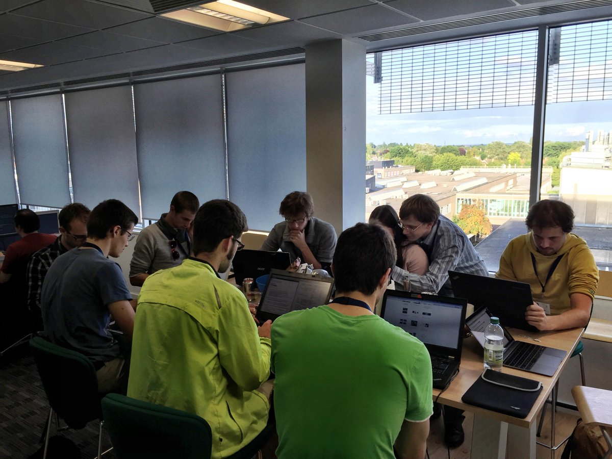
I was feeling a bit hypocritical for missing the sprints this year, since I had to run off before the Sunday. Emmanuelle Gouillart, another scikit-image core dev, suggested having a small, unofficial sprint on Friday evening. It grew and grew into a group of about 30 people (including about 10 new to sprinting) who all gathered at the Enthought Cambridge office to work on scikit-image or the SciPy lecture notes. A brilliant experience.

(By the way, nothing creepy going on with that dude hunching over one of our sprinters — that’s just husband-and-wife team Olivia and Robin Wilson! ;)

Final thoughts

As usual, I learned heaps and had a blast at this SciPy conference (my fourth). I hope it will remain a yearly ritual, and I hope someone reading this will give it a try next year!

Calling out SciPy on diversity (even though it hurts)

Over the past few weeks, I’ve been heavily promoting the SciPy conference, a meeting about scientific programming in Python. I’ve been telling everyone who would listen that they should submit a talk abstract and go, because scientific programming is increasingly common in any scientist’s work and SciPy massively improves how you do that.

I have also been guiltily ommitting that the speaker and attendee diversity at SciPy is shockingly bad. Last year, for example, 15% of attendees were women, and that was an improvement over the ratio three years ago, when just 3% (!!!) were women.

I rationalised continuing to promote this conference because there was talk from past organisers about making efforts to improve. (And indeed, the past three years have been on an upward trajectory.)

A couple of days ago, however, the full list of keynote speakers was announced, and lo and behold, it’s three white guys. I have to acknowledge that they are extremely accomplished in the SciPy universe, and, if diversity were not more generally a problem at this conference and in tech in general, I wouldn’t bat an eye. Excellent choice of speakers, really. Looking forward to it.

But diversity is a problem. It’s an enormous problem. I’m inclined to call it catastrophic.

Let me try to quantify it. Men and women are equally capable scientific programmers. So out of a total pool of 100 potential SciPy attendees/contributors, 50 are women and 50 are men. Now, let’s assume the male side of the community is working at near-optimum capacity, so, 50 of 50 those men are at SciPy. 15% of attendees being women means just 9 of the 50 potential female contributors are making it out to the conference (9/59 ≈ 15%). Or, slice it another way, a whopping (50 – 9) / 50 = 82% of women who could be contributing to SciPy are missing.

Now, think of where we would be if we took 82% of male science-Pythonistas and just erased their talks, their discussions, and their code contributions. The SciPy ecosystem would suck. Yet that is exactly how many coders are missing from our community.

Now, we can sit here and play female conference speaker bingo until the cows come home to roost, but that is missing the point: these are all only excuses for not doing enough. “Not my fault” is not good enough anymore. It is everyone’s fault who does not make an active and prolonged effort to fix things.

The keynote speakers are an excellent place to make a difference, because you can eliminate all sorts of confounders. I have a certain sympathy, for example, for the argument that one should pick the best abstracts/scholarship recipients, rather than focus on race or gender. (Though the process should be truly blind to remove pervasive bias, as studies and the experience of orchestra auditions have repeatedly shown.) For keynotes though, organisers are free to pursue any agenda they like. For example, they can make education a theme, and get Lorena Barba and Greg Wilson in, as they did last year.

Until the gender ratio begins to even remotely approach 1:1, diversity as an agenda should be a priority for the organisers. This doesn’t mean invite the same number of women and men to give keynotes. This means keep inviting qualified women until you have at least one confirmed female keynote speaker, and preferably two. Then, and only then, you can look into inviting men.

Women have been found to turn down conference invitations more often than men, irrespective of ability or accomplishment. I don’t know why, but I suspect one reason is lack of role models, in the form of previous female speakers. That’s why this keynote roster is so disappointing. There’s tons of accomplished female Pythonistas out there, and there would be even more if we all made a concerted effort to improve things.

I don’t want to retread the same territory that Jonathan Eisen (@phylogenomics) has already covered in “Calling attention to meeting with skewed gender ratios, even when it hurts“. In particular, see that article for links to many others with ideas to improve gender ratios. But this is my contribution in the exact same series: I love SciPy. See my previous posts for illustration.

Even looking back at my recent post, when I looked for a picture that I thought captured the collegial, collaborative feel of the conference, I unintentionally picked one featuring only men. This needs to improve, massively, if I’m going to keep supporting this conference. I really hope the organisers place diversity at the centre of their agenda for every decision going forward.

I thank Jonathan Eisen, Andy Ray Terrel, and April Wright for comments on earlier versions of this article.